Memory and Linux Processes

Physical Memory and Virtual Memory

The CPU of the computer is responsible for executing instructions (machine code). These instructions, as well as the data used by these instructions, should be placed in the physical memory (which is on the actual memory chip).  Each byte in the physical memory is accessed through a physical address. The physical address is placed in the memory address register (MAR) when writing or reading to/from memory. The size of the MAR and address bus determine the range of addresses that can be used. For example, if MAR is 32 bits, then addresses from 0 to 0xFFFFFFFF (up to 4GB) can be accessed.

(https://archive.cnx.org/contents/6876272b-9b8f-463c-848b-1d388dccf776@1/module-5)

Modern computer architectures however provide a virtual or logical memory view to the CPU. The CPU accesses each byte through a virtual or logical address. The range of virtual addresses is usually the same as the range of the physical addresses, although the actual amount of physical memory may be less or more than the addressable range.

Virtual addresses must eventually be translated to physical addresses to access instructions and data from the physical memory. This translation/mapping is technically called address binding. The translation is performed by the Memory Management Unit (MMU) hardware component. Schemes such as segmentation and/or paging are often used to support different features and needs, such as protection . The operating system also performs some operations related to this address translation by invoking specialized CPU instructions.

(https://upload.wikimedia.org/wikipedia/commons/thumb/d/dc/MMU_principle_updated.png/325px-MMU_principle_updated.png)

Application programmers need only to concern themselves with the virtual memory. Kernel developers, however, need to be concerned with both virtual and physical memory as part of implementing the memory management component of the operating system.

Having a virtual memory view provides flexibility, especially in multiprogramming and timesharing operating systems. It allows a process to "believe" that it has exclusive and full access to the entire physical memory, even though it does not. Also, virtual memory allows processes to access code and data that are in secondary storage (disk) as if they are in physical memory through a scheme called swapping.

Process Memory Map in Linux (Ubuntu 16.04 x86_64, GCC 5.4.0)

When writing C programs, variables are used to hold data and functions are used to implement operations. The variables and functions have names, which are symbolic. In compiler design, names are generally called symbols. Consider a payroll program, the variable named age can be used to hold the age of an employee. Also, the function named compute_salary can be used to perform the operation of computing the salary of an employee.

When a C program is compiled and linked, the variables and functions are converted to memory locations/addresses(in virtual memory) and machine code(object code) respectively.  Variable names and function names become memory addresses and are stored in a symbol table. The result of this conversion is stored in an executable file (aka program binary image). The executable file is what is usually run. Executable file format is usually dependent on the operating system. In Linux for example, ELF is the standard format for executable files.

Running a program actually means the loader reading the executable file and creating a process for it. When the executable file is loaded by the operating system for execution, for example via the exec() system call in Linux, the operating system allocates a portion of memory in an area dedicated for user processes.  The data and instructions are read from the executable file and placed in the allocated memory in locations which are also specified(in the symbol table) from  the executable file. Again, it is emphasized that the memory locations being referred to here is in virtual memory. Once the data and instructions are in memory, a new process control block(PCB) is created representing the process. The allocated memory becomes the process' memory map or address space and is usually a field in the PCB. The process is then scheduled for execution.

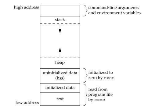
A process' memory map is divided into sections which serve different purposes. A typical memory map is shown below. The text section for instructions, the data section for initialized data, the bss section for uninitialized data, the stack section for function calls (and traditionally, parameters), and the heap section for dynamically allocated memory (via the function malloc()). Some of these sections are already defined during the compilation and linking process. Although it appears below that the memory is contiguous in virtual memory, it may not be the case in the corresponding physical memory.

(https://www.hackerearth.com/practice/notes/memory-layout-of-c-program/)

The example C program below will illustrate in what section of a process' memory map the different symbols are placed. Download binding.c, create an object file and executable file [1]. Run the executable several times and observe which variables change in address. The variables are so named to show in which section they will reside.

Compile time (output is object file):
$ gcc -fno-common -c -o binding.o binding.c

Link time (output is executable file):
$ gcc -fno-common -o binding.exe binding.c

Run time (a process is created) :
$ ./binding.exe

Next, examine the symbol table of the object file and the executable file. The first column refers to the assigned address and the fourth column refers to the assigned section.
$ objdump -t binding.o 
$ objdump -t binding.exe

Compare the entries for some of the symbols in the object file and executable file. Which file contains an address for the symbol, the object file or the executable file?
$ objdump -t binding.o | grep data_global_initialized_nonzero
$ objdump -t binding.exe | grep data_global_initialized_nonzero 

$ objdump -t binding.o | grep -w bss_global
$ objdump -t binding.exe | grep -w bss_global

$ objdump -t binding.o | grep -w text_func
$ objdump -t binding.exe | grep -w text_func

Can the symbols that start with stack_ and those stored in the heap be found?No. The stack section and heap section are allocated at run time.

Let us look where each of the sections start in memory and the symbols in each section.
$ objdump -t binding.exe | grep -w .text
$ objdump -t binding.exe | grep -w .data
$ objdump -t binding.exe | grep -w .bss

We will now use GDB to examine the process address space at run time. GDB will allow us to examine the state of the execution by allowing us to run one instruction at a time. (Try to compare the addresses at link time and at run time. Are they the same?)
$ gdb ./binding.exe
(gdb) set disassembly-flavor intel
(gdb) b main+99
(gdb) r
(gdb) disas main
(gdb) info proc mapping
   
Study the memory map. Notice that there is no heap section yet. This is because no call to malloc() has been made yet.
(gdb) ni +6
(gdb) disas main
(gdb) info proc mapping

The heap section is now present. Let us look for the variables in the sections.
(gdb) find 0x601000,+0x1000,"JACH_IN_DATA"
(gdb) find 0x601000,+0x1000,"JACH_IN_BSS"
(gdb) find 0x602000,+0x21000,"JACH_IN_HEAP"
(gdb) find 0x7ffffffde000,+0x21000,"JACH_IN_STACK_LOCAL"

How about the parameter?Is it in the stack?
(gdb) find 0x7ffffffde000,+0x21000,"JACH_IN_STACK_PARAM"

The string is not in the stack! It is in the text section! Traditionally however, parameters are pushed to the stack.
(gdb) find 0x400000,+0x1000,"JACH_IN_STACK_PARAM"

Finally, run the process to completion.
(gdb) c
(gdb) quit 

Conclusion

This post discussed some concepts in memory management in relation to C programs and Linux processes.

Figure 1. Sample Memory Map (no heap section yet)

Read More

Build-and-Run: From C Programs to Linux Processes

A typical C program undergoes several transformations before it becomes a running process. This post illustrates these transformations. We are given two source files and one header file. These steps were tested on a x86-64 Ubuntu 16.04 machine. The figure below (from https://www.hackerearth.com/practice/notes/build-process-cc/ ) summarizes the steps.

 

//sum.h
#ifndef __SUM_H_
int sum(int, int);
#endif

------------------

//sum.c
#include "sum.h"
int sum(int a, int b){
   return a+b;
}

------------------

//main.c
#include <stdio.h>
#include "sum.h"

int a=3;
int main(){
   int b=4;
   printf("a+b=%d\n",sum(a,b));
   return 0;
}
-----------------



Create sum.o
----------------------
1. Preprocess
$ cpp -o sum.i sum.c

2. Generate asm code from preprocessed
$ gcc -S -o sum.S sum.i

3. Create object file
$ as -o sum.o sum.S

4. Examine object file
$ objdump -x -d -M intel sum.o | less


Create main.o
-----------------------
1. Preprocess
$ cpp -o main.i main.c

2. Generate asm code from preprocessed
$ gcc -S -o main.S main.i

3. Create object file
$ as -o main.o main.S

4. Examine object file
$ objdump -x -d -M intel main.o | less   

Create the final executable main.exe
------------------------------------------------------------
1. Link main.o sum.o and system libraries
$ ld -o main.exe main.o sum.o -dynamic-linker /lib64/ld-linux-x86-64.so.2 /usr/lib/x86_64-linux-gnu/crt1.o /usr/lib/x86_64-linux-gnu/crti.o /usr/lib/gcc/x86_64-linux-gnu/5/crtbegin.o -lc /usr/lib/gcc/x86_64-linux-gnu/5/crtend.o /usr/lib/x86_64-linux-gnu/crtn.o

2. Examine object file
$ objdump -x -d -M intel main.exe | less

3. Use gdb to load the program and create a process
$ gdb ./main.exe
(gdb) set disassembly-flavor intel
(gdb) b main
(gdb) r
(gdb) disas main
(gdb) info proc all
(gdb) c
(gdb) quit

Read More

Expenses and SQL

I've been using the free version of Expense Manager to keep track of my expenses last 2017 and luckily I was able to make complete entries for the whole year. This year I plan to set a monthly budget and try to stick to it and I will be using last year's data.

Expense Manager uses sqlite as storage and it has an option to backup the data either as raw sqlite data or csv. Instead of using the raw sqlite data backup, I created a new database (using sqlite3)  and created the expenses schema is below. 

CREATE TABLE expenses(
   date_incurred DATE, 
   amount NUMERIC(8,2),
   category VARCHAR(27),
   description VARCHAR(24)
);

After preprocessing the csv file by removing unneeded columns, sample insert statements generated are shown below.

INSERT INTO expenses(date_incurred,amount,category,description) VALUES ('2017-01-01',-55,'Snacks',NULL);
INSERT INTO expenses(date_incurred,amount,category,description) VALUES ('2017-01-01',-21,'Transportation',NULL);
INSERT INTO expenses(date_incurred,amount,category,description) VALUES ('2017-01-02',-1150,'Others','radio');
INSERT INTO expenses(date_incurred,amount,category,description) VALUES ('2017-01-02',-66,'Others','battery');
INSERT INTO expenses(date_incurred,amount,category,description) VALUES ('2017-01-02',-1700,'Others','bag');
INSERT INTO expenses(date_incurred,amount,category,description) VALUES ('2017-01-02',-500,'Dinner',NULL);

Some of my expense categories:

Snacks
Transportation
Others
Dinner
Medicines and Supplements
Breakfast
Lunch
Groceries
Apartment Rent
Cable/Internet
Laundry
Water
Cellphone Load
Haircut
Clothing
Mom Allowance
Books and Reading Materials 
Rest and Recreation
 
Now to answer some of the interesting questions.

What was my total expenses for February 2017?
>select sum(amount) from expenses where date_incurred>="2017-02-01" and date_incurred<="2017-02-28";

What was my total expense for 2017?
>select sum(amount) from expenses;

What are the categories of my expenses?
>select distinct category from expenses;

How many times did I pay my apartment rent in 2017?
>select count(amount) from expenses where category="Apartment Rent";

How much did I pay for breakfast in 2017?
>select sum(amount) from expenses where category="Breakfast";

How much is my expense per month in 2017?
>select strftime('%m',date_incurred) as month, sum(amount) as amt from expenses where strftime('%Y',date_incurred)='2017' group by month;

How much did I spend for lunch each month, total and average, in 2017?
>select strftime('%m',date_incurred) as month, sum(amount) as amt,avg(amount) as mean from expenses where strftime('%Y',date_incurred)='2017' and category="Lunch" group by month order by amt;

What is the average amount I spent for lunch in 2017?
>select avg(amount) from expenses where category='Lunch';

My budget for snacks for one month should be.
>select avg(amount)*30 from expenses where category='Snacks';

Read More

Highlights of my academic life in 2017

• Presented a paper in PCSC 2017
• Presented a paper in NCITE 2017
• Started teaching again after four years of being on study leave
• Taught a new course: Computer and Network Security
• Attended technical conferences sponsored by private companies
• Helped SRG members in their SP/thesis proposals, undergraduate and graduate
• Participated in the 2017 ACM-ICPC Asia-Manila Regionals
• Presented in SESAM's graduate seminar on Space Science
• Maintained the operation of the Peak-Two Cloud
• Learned new Web Dev Technologies

Read More

2017 ACM-ICPC Regionals Asia-Manila Experience

We have two teams from ICS for this event held at Ateneo de Manila University last December 13-15, 2015. It is good to have been part of this event again after a long break. Thanks to Sir Clinton Poserio, head coach of the Eliens team, for inviting me. The ICS alumni have been a great help in providing financial support. A team from National University of Singapore was the winner in the competition. The top team from the Philippines was from the Ateneo de Manila University. The contest website is here.

Read More